For a while I’ve used JMP for data analysis professionally. Recently we’ve been talking about experiment design and statistical power at work and during some of these discussions I decided it might be good if I knew how to do some R. The learning curve is OK but there’s a lot of kind of magical behavior that I don’t really get yet.
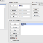
So far I’m working on getting a handle on linear models. JMP has a dialog that is Analyze->Fit Model. It then gives you a nice little browsing interface and lets you build your model with the crosses and nesting and all that. Then you tell it what kind of model you want and what kind of report you’re interested in seeing and let it go. I have a sample dataset that has nothing to do with work that has a response variable “delta”, a couple of continuous variables that effect delta and then a nominal variable “coding” which is essentially, control / experimental. I’ve fit several different models to this data but knowing what I know about how I built the dataset, it makes sense to nest the continuous variables within “coding”. The report it produces has a lot of nicely formatted data and you can run additional tests and reports from within that.
R is a much more programmy kind of tool. It’s possible to get the same model in one line of code.
> lmfit <- lm(data$delta ~ data$coding + data$dt*data$coding + data$dt2*data$coding, read.csv("derp.csv"))
But then you have a result object that you interrogate for information. I'm still struggling with the data structures R presents. The way you index into them to get at specific data really hasn't clicked yet and I find myself fumbling around in the terminal a lot. This is what it looks like when you ask it for the linear model and a summary thereof.
 > lmfit

Call:

lm(formula = data$delta ~ data$coding + data$dt * data$coding +

    data$dt2 * data$coding, data = read.csv("derp.csv"))
Coefficients:
(Intercept) data$codingb data$dt
2.15264 0.01773 0.75516
data$dt2 data$codingb:data$dt data$codingb:data$dt2
0.51304 1.67854 0.96067
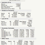
> summary(lmfit)
Call:
lm(formula = data$delta ~ data$coding + data$dt * data$coding +
data$dt2 * data$coding, data = read.csv("derp.csv"))
Residuals:
Min 1Q Median 3Q Max
-2.25889 -0.22361 0.03567 0.39381 2.18111
Coefficients:
Estimate Std. Error t value Pr(>|t|)
(Intercept) 2.15264 0.37886 5.682 2.23e-06 ***
data$codingb 0.01773 0.55084 0.032 0.97452
data$dt 0.75516 0.21063 3.585 0.00104 **
data$dt2 0.51304 0.20672 2.482 0.01818 *
data$codingb:data$dt 1.67854 0.29369 5.715 2.02e-06 ***
data$codingb:data$dt2 0.96067 0.29090 3.302 0.00226 **
---
Signif. codes: 0 ‘***’ 0.001 ‘**’ 0.01 ‘*’ 0.05 ‘.’ 0.1 ‘ ’ 1
Residual standard error: 1.018 on 34 degrees of freedom
Multiple R-squared: 0.9205, Adjusted R-squared: 0.9088
F-statistic: 78.75 on 5 and 34 DF, p-value: < 2.2e-16
It's not as pretty but all of the information is there. Also you can save everything as a script and rerun it if you get more data or a different dataset with the same columns. JMP also supports scripting but I honestly have never used it.
I do find R's form of the fit equation to be easier to understand but either way you have to make sense of the idea that "if experimental use these coefficients, if control use these others":
R:
(Intercept)           2.15264

data$codingb          0.01773

data$dt               0.75516

data$dt2              0.51304

data$codingb:data$dt  1.67854

data$codingb:data$dt2 0.96067
vs
JMP:
5.476 + Match( :coding, "a", (:dt - 1.3) * 0.755, "b", (:dt - 1.3) * 2.434)

      + Match( :coding,	"a", (:dt2 - 1.25) * 0.513, "b", (:dt2 - 1.25) * 1.474)

      + Match( :coding, "a", -1.700, "b", 1.700, . )